
How to Build a Machine Learning Model Fast: From Problem to Tested Baseline
The fastest reliable way to build a machine learning model is to start with a specific prediction problem, prepare labeled examples, separate training data from evaluation data, and fit a simple baseline with a library such as scikit-learn. Then measure whether the model makes better decisions than a trivial alternative before investing in complex algorithms or production infrastructure.
Quick answer: five rules for building a machine learning model fast
- Define the prediction before choosing an algorithm. Specify what you want to predict, when the prediction will be made and which business action it should support.
- Use a small, representative labeled dataset. Data quality, label reliability and feature availability matter more than starting with a complicated model.
- Split the data before preprocessing or training. Keep validation data for model decisions and a separate test set for the final evaluation.
- Compare against a simple baseline. A machine learning model must outperform an appropriate existing rule or trivial prediction to justify its extra complexity.
- Evaluate the cost of mistakes. Accuracy alone can hide false positives or false negatives that make a model unsuitable for the intended workflow.
For engineers and product founders, the fastest defensible approach is not the shortest path to a trained model. It is the shortest path to understanding whether useful prediction is possible with the information available at decision time. A model that trains successfully but relies on leaked information, unreliable labels or an inappropriate metric has not shown that it can solve the problem.
This guide includes a runnable Python classification example, a completed baseline comparison, a train/validation/test leakage checklist and a decision tree for choosing between batch predictions and an API.
Step 1: Define exactly what your machine learning model should predict
Before writing code, express the problem as a prediction target and a follow-up action. A broad goal such as “use AI to improve customer retention” is not specific enough to decide what data to collect or how to evaluate the result.
A better question is: “Using information available today, which customer accounts are likely to become inactive within the next 30 days, so that our team can decide whether to contact them?”
This statement establishes four parts of the project:
- Prediction unit: One customer account at a defined point in time.
- Target: Whether the account meets the agreed inactivity definition during the next 30 days.
- Available inputs: Information known at the prediction date, such as historical product activity or previous support interactions.
- Business action: Prioritize accounts for a suitable retention outreach process.
The inactivity definition must be explicit. For example, a business might define an inactive account as one with no qualifying product activity during a complete 30-day observation period. That definition will not suit every SaaS business, but it creates a label that can be evaluated.
Choose a problem type that matches the decision
| Business question | ML problem | Typical output | Useful evaluation approach |
|---|---|---|---|
| Will this customer become inactive? | Binary classification | Positive or negative class, optionally with a score | Precision, recall, false positives, false negatives and decision costs |
| How much demand should we expect? | Regression | Numerical prediction | Absolute error and the consequences of under- or overprediction |
| Which category does this request belong to? | Multiclass classification | One of several defined categories | Per-class error analysis and confusion matrix |
| Which items should we inspect first? | Ranking or classification | Priority score or ordered list | Performance among top-ranked items and workload constraints |
The worked example below uses binary classification. The same sequence of problem definition, honest evaluation and deployment planning applies to other machine learning tasks, although the models and metrics differ.
Step 2: Choose data that would exist when the prediction is made
Each training example needs inputs, called features, and an observed target, called a label. For supervised learning, historical examples must contain enough information to determine what actually happened after the prediction point.
Consider a hypothetical customer retention dataset:
| Field | Example meaning | Can it be used at prediction time? |
|---|---|---|
| account_id | Identifier for the customer account | Used for record identity and splitting; not automatically a predictive feature |
| prediction_date | Date the hypothetical prediction would have been made | Used to set the observation cutoff and evaluation design |
| active_days_last_30 | Number of active days before the prediction date | Yes, if the source data was available at that time |
| previous_support_tickets | Number of earlier support requests | Yes, if calculated only from events before the cutoff |
| subscription_age_days | Account age at prediction time | Yes, if defined consistently |
| inactive_next_30_days | Whether the account met the inactivity rule afterward | No. This is the target label, not an input feature |
| cancellation_recorded_after_prediction | Information entered after the prediction date | No. It would reveal future information unavailable to the model |
The key rule is simple: the model should not learn from information that would be unavailable when the real prediction is made.
Using a cancellation date recorded after the prediction point may produce excellent offline scores, but those scores would not reflect what the system can achieve when predicting future customer behavior. Google’s Machine Learning Crash Course is a useful free reference for the underlying concepts, including its module on datasets, generalization and overfitting, which covers preparing data for training and evaluation.
How much data do you need?
There is no universal minimum number of rows that guarantees a useful model. The amount needed depends on the frequency of the target outcome, feature quality, model complexity, variation in the population and the precision required from the evaluation.
For a first experiment, check whether the labeled examples cover both target classes and the situations in which the model will be used. If very few accounts ever become inactive, thousands of total records may still contain too few positive examples for a dependable assessment. If historical labels are inconsistent, collecting more of the same data may not fix the problem.
If usable labels do not exist, building a reliable labeling process may be more valuable than starting model training immediately.
Step 3: Split the data before training
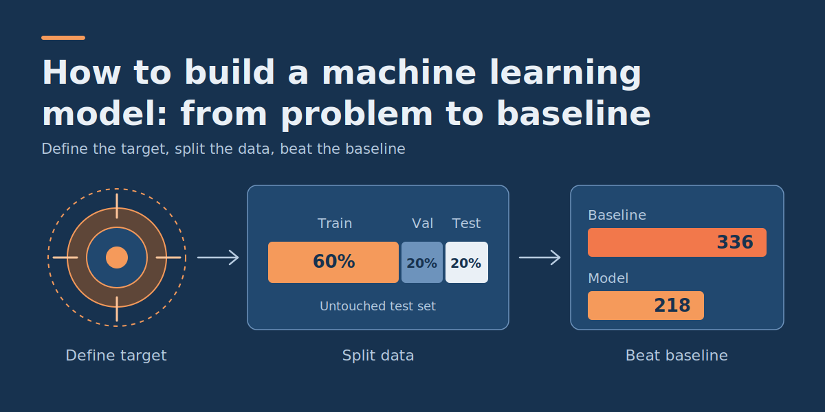
To evaluate a model honestly, keep the information used to fit it separate from the information used to judge it. For a straightforward dataset of independent examples, an initial split can use three partitions:
| Subset | Illustrative share | Purpose |
|---|---|---|
| Training | 60% | Fit preprocessing transformations and model parameters |
| Validation | 20% | Choose between candidate approaches or decision thresholds |
| Test | 20% | Perform a final evaluation after model choices are fixed |
These proportions are a demonstration, not a universal recommendation. The right design depends on the number of examples and, more importantly, on how data will arrive in the real application.
When a random split is the wrong choice
A random row-level split can exaggerate performance when records are related or when the task predicts future events.
- Time-dependent predictions: Train on earlier periods and evaluate on later periods that would not have been known during training.
- Repeated customer records: Use grouping when the intended evaluation requires unseen customers rather than new records from customers already in training.
- Duplicate or near-duplicate examples: Prevent effectively identical information from appearing in both training and evaluation subsets.
- Label observation windows: Make sure outcomes are fully observed and that overlapping windows do not reveal information across a split.
The code in the next section uses independent synthetic rows, so a stratified random split is appropriate for that demonstration. For a real future-inactivity predictor, a time-based design may be more realistic. Where both time and account grouping matter, account for both in the evaluation plan.
Step 4: Build a working machine learning baseline in Python
Now create and test a binary classifier using scikit-learn. The example is small enough to run locally or in a notebook without a GPU, cloud service or external dataset.
It uses 1,000 synthetic examples with six numerical features, and approximately 20% belong to the positive class. The generated features have no real customer meaning, so the results demonstrate the technical workflow rather than the predictive performance of a real retention product.
Two approaches are compared:
- Dummy baseline: Always predict the most common class observed during training.
- Logistic regression: Learn a relationship between the numerical features and the target.
Logistic regression is a reasonable first classifier for a small numerical tabular problem because it is relatively simple and provides class scores. A complex neural network is unnecessary for this demonstration.
Install the dependency
python -m pip install scikit-learnSave the following code as baseline.py or run it in a Python notebook.
Complete runnable example
from sklearn.datasets import make_classification
from sklearn.dummy import DummyClassifier
from sklearn.linear_model import LogisticRegression
from sklearn.metrics import confusion_matrix
from sklearn.model_selection import train_test_split
from sklearn.pipeline import make_pipeline
from sklearn.preprocessing import StandardScaler

# Synthetic data only; not actual customer information.
# Class 1 represents a hypothetical need for outreach.
X, y = make_classification(
    n_samples=1000,
    n_features=6,
    n_informative=4,
    n_redundant=0,
    weights=[0.8, 0.2],
    flip_y=0.03,
    random_state=42,
)

# First reserve an untouched 20% test set.
X_work, X_test, y_work, y_test = train_test_split(
    X, y,
    test_size=0.20,
    stratify=y,
    random_state=42,
)

# Split the remainder into 60% training and 20% validation.
X_train, X_val, y_train, y_val = train_test_split(
    X_work, y_work,
    test_size=0.25,
    stratify=y_work,
    random_state=42,
)

# Baseline: predict the most common training label.
baseline = DummyClassifier(
    strategy="most_frequent"
).fit(X_train, y_train)

# Preprocessing is fitted only on training data.
model = make_pipeline(
    StandardScaler(),
    LogisticRegression(max_iter=1000),
)
model.fit(X_train, y_train)

# Illustrative decision costs:
# False positive: 2 loss units.
# False negative: 8 loss units.
def report(y_true, y_pred):
    tn, fp, fn, tp = confusion_matrix(
        y_true, y_pred, labels=[0, 1]
    ).ravel()

    return {
        "TP": int(tp),
        "FP": int(fp),
        "FN": int(fn),
        "TN": int(tn),
        "loss_units": int(2 * fp + 8 * fn),
    }

# Choose a threshold using validation data only.
validation_scores = model.predict_proba(X_val)[:, 1]
thresholds = [0.20, 0.35, 0.50, 0.65]

selected_threshold = min(
    thresholds,
    key=lambda t: report(
        y_val, validation_scores >= t
    )["loss_units"],
)

print("Split sizes:", len(y_train), len(y_val), len(y_test))
print("Chosen validation threshold:", selected_threshold)

print(
    "Validation baseline:",
    report(y_val, baseline.predict(X_val)),
)
print(
    "Validation model:",
    report(y_val, validation_scores >= selected_threshold),
)

# Final test: do not retune after seeing these results.
print(
    "Test baseline:",
    report(y_test, baseline.predict(X_test)),
)

test_scores = model.predict_proba(X_test)[:, 1]
print(
    "Test model:",
    report(y_test, test_scores >= selected_threshold),
)
What the code does
- Generates labeled data:
make_classificationproduces numerical examples and binary labels. - Creates separate datasets: Training contains 600 rows, validation 200 and testing 200.
- Fits a dummy baseline: The simplest comparison predicts the majority class.
- Trains a logistic regression pipeline: The pipeline fits scaling parameters and the classifier on the training subset only.
- Selects a decision threshold: Four candidate thresholds are compared on validation data using the illustrative false-positive and false-negative costs.
- Evaluates the untouched test subset: The chosen threshold and trained models are evaluated without further adjustment.
Using a Pipeline keeps preprocessing and the estimator together. According to the scikit-learn common pitfalls guide, a pipeline makes it easier to chain transformations with estimators and reduces the chance of forgetting a transformation, and it also helps prevent leaking test data into training.
Actual output from the worked example
The script was executed with the stated random seed (scikit-learn 1.8.0). Its output was:
Split sizes: 600 200 200
Chosen validation threshold: 0.35

Validation baseline:
{'TP': 0, 'FP': 0, 'FN': 42, 'TN': 158, 'loss_units': 336}

Validation model:
{'TP': 18, 'FP': 11, 'FN': 24, 'TN': 147, 'loss_units': 214}

Test baseline:
{'TP': 0, 'FP': 0, 'FN': 42, 'TN': 158, 'loss_units': 336}

Test model:
{'TP': 17, 'FP': 9, 'FN': 25, 'TN': 149, 'loss_units': 218}
These are reproducible results from generated data, not a benchmark of real customer inactivity prediction. Numerical results can vary with library versions and environments.
The example demonstrates the mechanics of choosing a threshold on validation data and then evaluating on a held-out test set. It does not establish that the chosen threshold, model or artificial cost weights would work in a real business.
Step 5: Evaluate model performance against the baseline
Training completes the computation; evaluation determines whether the output is useful. For binary classification, a confusion matrix separates four outcomes:
| Outcome | Meaning in the illustrative example |
|---|---|
| True positive (TP) | The model flags an account that actually belongs to the positive class |
| False positive (FP) | The model recommends outreach for an account that does not belong to the positive class |
| False negative (FN) | The model misses an account that belongs to the positive class |
| True negative (TN) | The model correctly leaves an account unflagged |
The test set contains 42 positive and 158 negative examples. The majority-class baseline labels every case negative, so it misses all 42 positives while correctly identifying all 158 negatives. The trained classifier, using the validation-selected threshold of 0.35, finds 17 of the 42 positives and generates nine false positives.
Compare the results
| Test measure | Majority baseline | Trained model |
|---|---|---|
| Correct predictions | 158 of 200 | 166 of 200 |
| Accuracy | 79% | 83% |
| True positives | 0 | 17 |
| False positives | 0 | 9 |
| False negatives | 42 | 25 |
| Recall | 0% | 40.5% |
| Illustrative total loss units | 336 | 218 |
The model beats the majority baseline on this synthetic test set by both accuracy and the assumed loss calculation. However, it still misses 25 of 42 positive examples. Whether that is acceptable depends on the intended operation. If a missed positive case has serious consequences, this model may be unsuitable even though it improves on the trivial baseline.
This is why accuracy should not be the only metric. Google’s Machine Learning Crash Course covers this in its classification module, which introduces thresholding, confusion matrices and metrics such as accuracy, precision, recall and AUC.
Evaluate the cost of false positives and false negatives
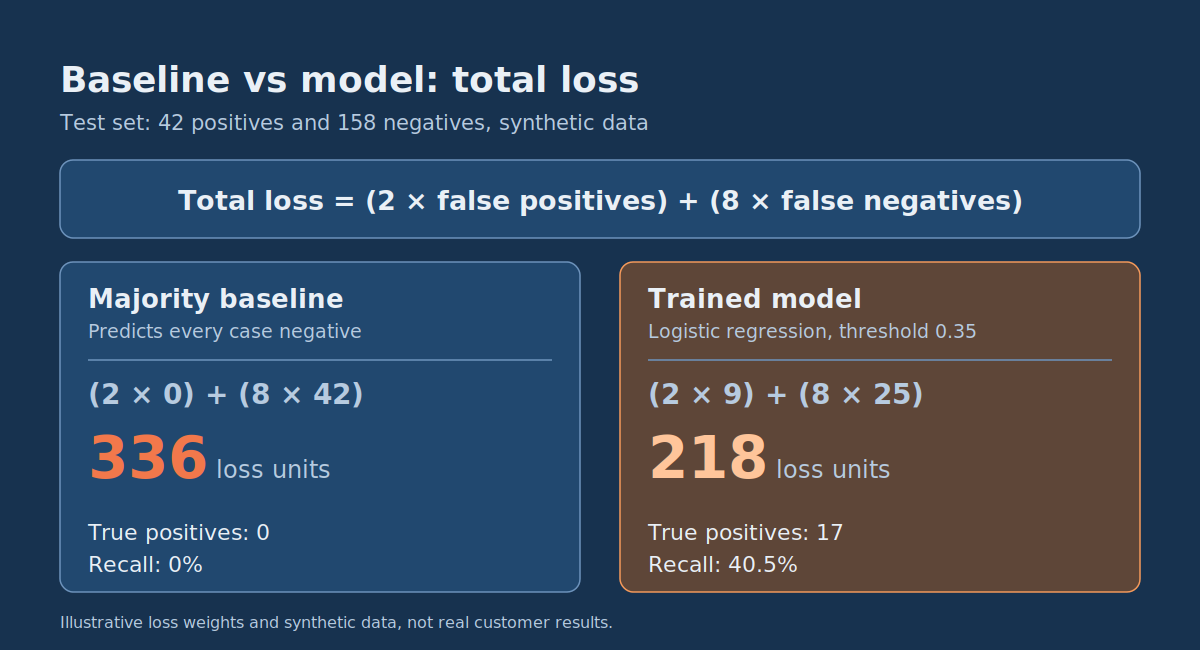
In the code, a false positive costs two hypothetical loss units and a false negative costs eight. These figures are illustrative preferences, not measured monetary values.
Total loss = (2 × false positives) + (8 × false negatives)
For the trained model on the test set: (2 × 9) + (8 × 25) = 218 loss units.
For the majority baseline: (2 × 0) + (8 × 42) = 336 loss units.
In a real retention workflow, contacting an account has a cost, but a missed prediction does not necessarily imply a fixed financial loss. Not every flagged account would respond to outreach, and a prediction alone does not prove that contacting the customer will change the outcome.
Replace the illustrative loss assumptions with a business-approved decision model. If the intervention itself needs evaluation, design an appropriate experiment rather than treating predictive accuracy as proof of business impact.
Step 6: Check for data leakage before trusting the result
Data leakage occurs when a model is built using information that would not be available at prediction time. According to the scikit-learn documentation on data leakage, this produces overly optimistic performance estimates and poorer results on genuinely new data in production.
Leakage is not limited to accidentally including the target column as a feature. It can also arise from preprocessing, duplicate records, time-dependent information or an evaluation process that repeatedly adapts to test-set results.
The same documentation states a general rule: never call fit on the test data. It also shows how serious preprocessing leakage can be. On a dataset of completely random features and labels, running feature selection on all the data before splitting produced an accuracy of 0.76, while doing it correctly on the training data alone gave about 0.5, which is the expected chance level.
Train/validation/test leakage checklist
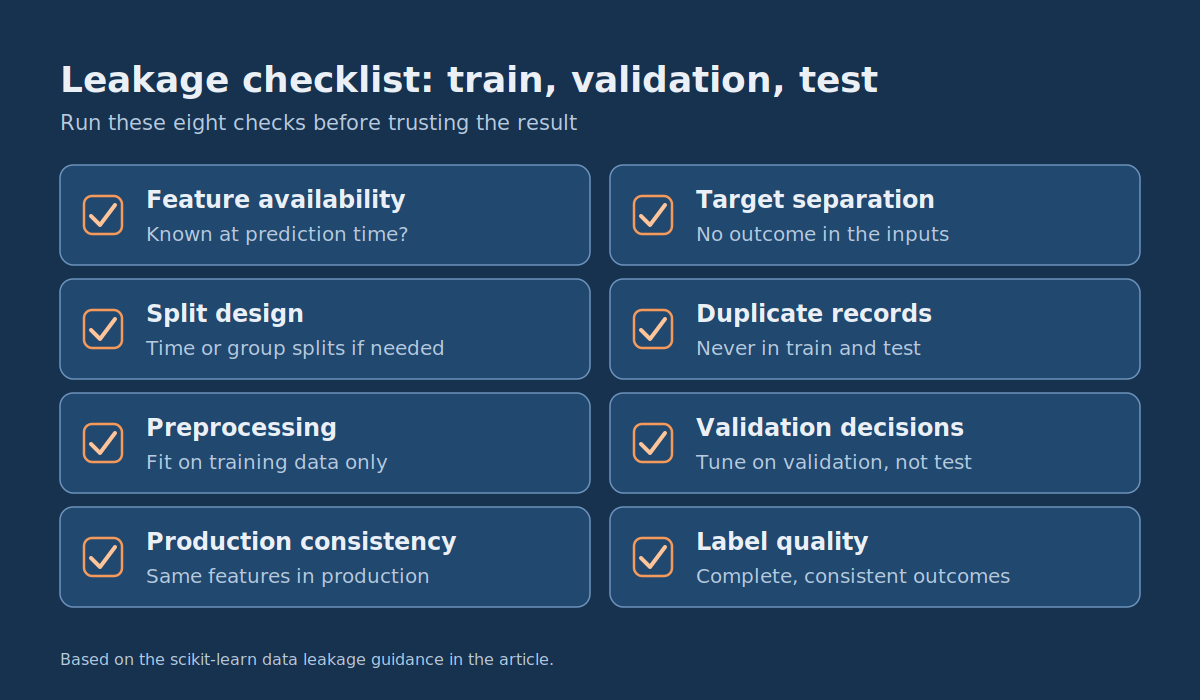
| Check | Failure to prevent | What to do |
|---|---|---|
| Feature availability | Training uses information recorded after the prediction point | Verify when each feature becomes available in the actual system |
| Target separation | The target or a direct proxy appears among the input features | Inspect feature definitions and remove outcome-derived information |
| Split design | Related records or future information cross evaluation boundaries | Use temporal or group-based splits when the prediction scenario requires them |
| Duplicate records | The same observation appears in training and testing | Establish deduplication rules and prevent shared underlying observations |
| Preprocessing | Imputation, scaling or feature selection is fitted on held-out data | Fit preprocessing only on the training subset, preferably inside a pipeline |
| Validation decisions | Thresholds or model settings are selected using the final test set | Use training and validation data for selection; reserve test data for final evaluation |
| Production consistency | Training and production construct features differently | Define and test a consistent input schema and transformation process |
| Label quality | Targets are incomplete, inconsistent or not yet fully observed | Check label generation, observation windows and uncertain cases |
A useful review question: “Could the production application have calculated this exact feature, with the same meaning and available information, at the moment it needed to predict?” If not, the feature should not be used in that form.
Why using the test set repeatedly is a problem
Suppose the model performs poorly on the test set, and the team changes the threshold, tries several features and selects a new algorithm based on those results. The test set is now influencing development decisions. Repeating that process produces an overly optimistic estimate, because development has adapted to examples that were supposed to remain unseen.
Use validation data for such decisions. Once the approach is fixed, evaluate the held-out test set. If the result is inadequate and development resumes, recognize that another trustworthy final evaluation may require newly held-out data or a revised evaluation design.
Step 7: Adapt the example to your own labeled dataset
The synthetic example uses six numerical columns with no business meaning. To build something useful, replace them with real features and labels that follow the definitions from Steps 1 and 2. For example, suppose you have a CSV file containing one appropriately constructed historical prediction snapshot per row:
import pandas as pd

df = pd.read_csv("labeled_accounts.csv")

feature_columns = [
    "active_days_last_30",
    "previous_support_tickets",
    "subscription_age_days",
]

X = df[feature_columns]
y = df["inactive_next_30_days"].astype(int)
This snippet replaces the synthetic data generation. It assumes the CSV already contains valid numeric features and a binary target with no missing labels. It does not automatically make the dataset safe to use.
Before applying the rest of the training code:
- Confirm that the target describes the intended future observation window.
- Check that each input field was available by its prediction timestamp.
- Decide whether a random split is appropriate or whether the evaluation needs time-based or account-based separation.
- Review missing values, categorical fields, units and outliers.
- Add training-only preprocessing for missing or categorical data when necessary.
- Replace the example loss weights with decision criteria appropriate to the actual workflow.
If the real dataset contains missing values, the StandardScaler and classifier pipeline may need an imputation step. If it contains categories, a categorical encoding step may also be required. Keep those learned transformations inside the training pipeline instead of applying them to the full dataset before evaluation.
For an initial real-world experiment, avoid creating dozens of engineered features without a reason. Start with a small, clearly understood set and determine whether it provides a measurable advantage over the baseline.
Step 8: Decide whether the model needs batch predictions or an API
A trained model is not automatically a deployable machine learning product. Once offline testing is complete, the next question is how predictions will be used. The simplest viable delivery method depends on when the prediction is required.
Deployment decision tree
START: When does the application need a prediction?
|
+-- At a scheduled time?
|   |
|   +-- YES -> Batch prediction
|       |
|       +-- Read an approved input dataset
|       +-- Run the validated model
|       +-- Save predictions to a controlled destination
|       +-- Let existing workflows consume the results
|
+-- Immediately after a user or system event?
    |
    +-- YES -> Online prediction interface
        |
        +-- Validate the request schema
        +-- Apply the same feature transformations
        +-- Run the model
        +-- Return a result with appropriate error handling
        +-- Monitor reliability and response times
Batch predictions: often the simpler first release
If customer account scores only need to be updated once a day, a scheduled batch process may be sufficient. A minimal batch workflow can:
- Read approved account features from the reporting or application database.
- Validate the inputs and construct features using the agreed definitions.
- Run the trained model for eligible accounts.
- Write account identifiers, scores, model version and prediction timestamps to an authorized destination.
- Make those scores available to the existing customer operations process.
Batch processing avoids introducing a network prediction service when predictions do not need to be immediate. It still needs scheduling, permissions, failed-run handling and monitoring, but those responsibilities may fit within existing application infrastructure.
API predictions: use when the result is needed on demand
An API is appropriate when a prediction must be generated in response to an application request or event, and a previously computed score is not current enough. For example, a product could request a prediction when an account enters a workflow that requires an immediate decision.
A minimal API contract for the synthetic demonstration might accept six ordered numerical features:
{
  "features": [0.2, -0.4, 1.1, 0.0, -0.7, 0.9]
}
This JSON is an illustrative input shape, not a running endpoint. A production interface should use documented, meaningful feature definitions and validate required fields, data types, ranges and authorization.
The serving process must apply the same fitted preprocessing as training. As the scikit-learn common pitfalls guide explains, transformations used during training must also be applied to production data, otherwise the feature space changes and the model cannot perform effectively. Never train a new scaler on each incoming request.
| Consideration | Batch prediction | Online API |
|---|---|---|
| Prediction timing | Scheduled or event-triggered groups of records | On-demand requests |
| Typical integration | Database tables, scheduled jobs or files | Application services and authenticated requests |
| Latency requirement | Results can be prepared before they are needed | Results must arrive within an application-specific response window |
| Infrastructure | Job execution, scheduling, storage and monitoring | Serving process, network interface, authorization and request monitoring |
| Main operational concern | Freshness, completeness and job failures | Availability, latency, load and invalid requests |
For an initial customer-retention workflow where staff review accounts each morning, batch predictions are a reasonable starting choice. Adding a real-time API would require evidence that immediate inference provides useful additional value.
Step 9: Check what is required before production deployment
A successful offline experiment establishes only part of the case for deployment. A production workflow must also be safe to operate and useful to the people consuming its results. Google’s Machine Learning Crash Course includes a module on production ML systems that covers how these components fit together; start from the course home page.
Model and input contract
Record the feature names, types, units, missing-value behavior and prediction-time availability. Ensure the deployed system uses the same preprocessing logic as the evaluated model. The anonymous columns in the example would need to be replaced by meaningful inputs before building a real customer-facing product.
Versioning and reproducibility
Keep a record of the training code, approved data snapshot or dataset reference, model configuration, evaluation results and software dependencies. Pin random_state to an integer, as the example does, if you need identical results across runs; scikit-learn’s default of None produces different results each time.
If you persist a trained model, remember that pickle-based formats, including joblib, can execute arbitrary code when loaded, and that package versions should match between training and deployment. Only load model artifacts from trusted, controlled sources.
Monitoring after deployment
Operational monitoring should cover more than whether the model process is running:
- Input failures: Invalid fields, missing values, schema changes and unexpected feature ranges.
- Prediction distribution: Changes in score patterns or the proportion of cases flagged for action.
- Model quality: Performance against outcomes once reliable labels become available.
- Business workflow: Whether predictions are used correctly and whether the intended decision process improves.
- System reliability: Failed jobs, API errors, latency and resource usage where applicable.
Not every prototype needs a dedicated MLOps platform. For a small batch system, an existing scheduler, clear logs, basic input validation and a named incident owner may be enough initially.
Common mistakes when trying to build ML models quickly
Choosing a complex algorithm before establishing a baseline
A sophisticated model is not automatically more useful than logistic regression, a decision tree or a well-designed business rule. Start with a baseline that tests whether the features contain useful signal. Explore more complex models when the simpler approach fails an important requirement that added complexity might realistically address.
If you later want to explore more advanced architectures, these deep learning project ideas show examples of more involved learning problems. They serve a different purpose from the fastest path to a defensible tabular baseline.
Reporting accuracy without examining the class distribution
If most examples belong to one class, a model that always predicts that class can look accurate while missing the outcomes the product is meant to identify. Our own example shows it: the majority baseline scores 79% accuracy and finds zero positives. Report class counts, a confusion matrix and metrics relevant to the decision.
Scaling or selecting features before splitting
Fitting preprocessing on the entire dataset lets evaluation information influence training. Separate the data first and use a pipeline for fitted preprocessing whenever practical.
Assuming a good offline result proves business value
A model can distinguish positive and negative examples without showing that acting on its predictions improves the business outcome. Predictive performance and intervention effectiveness are different questions. If the goal is better retention, evaluate the actual outreach process rather than assuming that identifying at-risk accounts causes them to stay active.
Building serving infrastructure before deciding how predictions are used
An API adds operational responsibilities. If predictions only need to be updated on a schedule, a batch process may meet the requirement with less implementation work. Choose infrastructure around the product workflow rather than defaulting to real-time inference.
How do you know whether your first ML prototype is good enough?
A first model is useful when it provides credible evidence for a product decision. That decision might be to run a limited operational pilot, collect better labels, revise the prediction target or stop the project. Use these release-readiness questions before investing in integration work:
| Question | Evidence required |
|---|---|
| Is the prediction problem well defined? | A target, observation window, prediction timestamp and intended action |
| Are labels and features usable? | Data-quality review and evidence that inputs exist when predictions are made |
| Is evaluation representative? | An appropriate split that addresses time, repeated entities and other dependencies |
| Does ML offer an advantage? | Comparison against a meaningful baseline using agreed metrics |
| Are mistakes acceptable? | Error analysis and an assessment of the actual consequences of false predictions |
| Is the proposed workflow practical? | A defined batch or API integration and a person or system responsible for acting on results |
| Can the model be maintained? | Input contract, reproducible implementation, monitoring and named operational ownership |
Failing one of these checks does not necessarily mean machine learning is impossible. It means the evidence is insufficient for the proposed next step. A promising test score accompanied by severe leakage risk is a reason to fix the evaluation, not to deploy. Likewise, a model that reliably predicts an outcome but does not affect any useful decision may not justify ongoing operational cost.
Frequently asked questions
What should I predict first when building a machine learning model?
Choose a narrow, observable outcome connected to an existing decision. The target should have a clear definition, reasonably reliable historical labels and input features available before the predicted outcome occurs. Good candidates often involve repetitive decisions with enough recorded history to evaluate. Avoid broad objectives such as predicting customer satisfaction or business success without defining exactly how they are measured.
How do I prevent data leakage?
Define the prediction timestamp, inspect feature availability and choose a split that reflects the real prediction setting. Keep related examples separated, fit preprocessing on training data only and reserve the final test set for evaluation after model and threshold choices are complete. A pipeline reduces some preprocessing risks, but it cannot detect business-level leakage caused by future information or an inappropriate split.
Do I need an API to create a machine learning application?
No. An application can use predictions generated by a scheduled batch job, a database-backed scoring process or an online prediction service. Use an API when predictions must be requested on demand and the application needs results immediately. Use batch processing when scores can be calculated ahead of time and consumed by an existing workflow.
Can I create a machine learning model without a GPU?
Yes. Many introductory classification and regression models train on ordinary CPUs, particularly with modest tabular datasets. The worked example uses scikit-learn and needs no GPU. More demanding models and larger datasets may require more resources, but that should follow the needs of the problem rather than determine the starting architecture.
When should I move from a baseline to custom ML development?
Move forward when a reliable evaluation shows the problem is worth pursuing and the remaining work requires integration, more complex data processing, specialized modeling or controlled production deployment. The next step is not necessarily a more advanced algorithm. It might be better feature collection, a revised metric, improved labeling or a small operational pilot.
Build a tested baseline before building the ML product
The fastest reliable way to create a machine learning model is to validate the prediction problem before investing in complexity. Define the target, use information available at decision time, split the data appropriately, train a simple model and compare it with a baseline using metrics that reflect the costs of errors.
The runnable example above shows the full evaluation path: synthetic data generation, training and validation, baseline comparison, threshold selection and one final test. Its results demonstrate a repeatable development method, not a production-ready customer prediction system.
For your own project, replace the synthetic data with appropriately labeled historical examples, choose a realistic evaluation split and decide what performance would justify the next stage. If a simple model cannot show useful signal, improving the data and problem definition is often more productive than training a larger model.
When a tested prototype needs custom integrations, a reliable prediction workflow or production engineering, DataColab can help scope the implementation around a defined business problem. Its custom AI and ML software services page gives context for evaluating that type of project, and its work on custom software development for business workflows covers connecting predictions to the systems your team already uses.
Pingback:Deep Learning Project Ideas: 12 Practical Projects with Datasets
Pingback:AI Training Data Labeling: Quality, Tools & Outsourcing
Pingback:Time Series Forecasting Explained: Baselines and Backtesting