
Time Series Forecasting: Baselines, Backtesting and Business Examples
What matters most about time series forecasting
- A forecast is only worth using if it beats a naive rule you could compute in a spreadsheet. In the worked example below, even the choice between two naive rules mattered: repeating last week’s value beat copying last year’s same week by a wide margin.
- Validation has to be chronological. In the same example, shuffled cross-validation reported a lower error (26.9) than the honest rolling-origin backtest (29.3) for the identical model, which is the flattery you get from letting a model train on the future.
- Percentage errors break when actual values reach zero. Report an error in real units (MAE), a total-volume percentage (WAPE), a scaled error (MASE) and a signed bias, and pick the headline number from the decision the forecast supports.
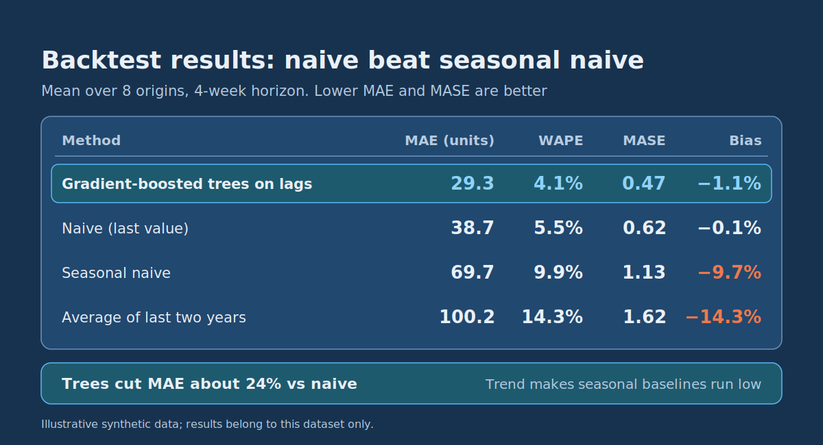
- Machine learning earned its place only after fair baselines were in place: gradient-boosted trees with lag features cut MAE by about 24% against the best naive rule on this illustrative dataset. That result belongs to this dataset and shouldn’t be assumed for yours.
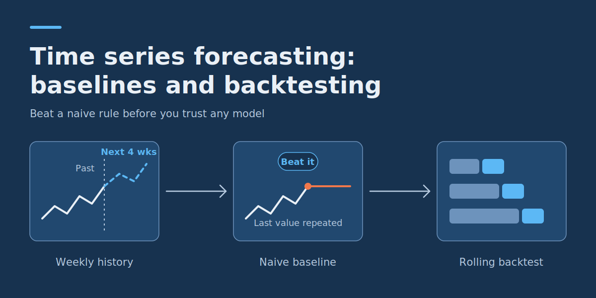
Time series forecasting means predicting future values of something measured at regular intervals, such as weekly orders, daily support tickets or hourly call volume, using its own history plus any drivers you know in advance, such as holidays or planned promotions. Producing a number is easy. The hard part for an analyst or operations planner is knowing whether that number is better than doing nothing clever, and avoiding the mistakes that make a weak model look strong. The short answer is to build a naive baseline first, evaluate every candidate with a rolling-origin backtest that never trains on information from after the forecast date, and score it with metrics that suit your data. Only then decide whether a more complex method is worth maintaining.
When time series forecasting pays off, and when it doesn’t
Forecasting earns its keep when a recurring decision depends on a future quantity. Typical cases include how much stock to order per product per week, how many agents to schedule for a support queue, how many pickers a warehouse needs on Thursday, and how much capacity to reserve for month-end processing. All of them share a repeated decision, a regular measurement and a horizon long enough to act on. The same logic applies to sensor and equipment readings, where IoT data analytics consulting can help you turn high-frequency device data into series that are clean enough to forecast.
Before touching data, write the forecasting question as three decisions: the grain (units per SKU per week), the horizon (the next 4 weeks) and the issue time (generated every Monday morning using data up to the previous Sunday). Everything later, from the train/test split to the metric, follows from these three lines. The worked example below uses exactly that spec.
Forecasting is a poor fit when there is too little history to see a seasonal cycle repeat, when the process just changed structurally (a new pricing model, a new channel), or when demand is so sparse that most periods are zero. In those situations a simple rule plus human judgement is often more honest than a model.
Trend and seasonality: what to check before choosing a method
Most business series combine a trend (a slow rise or fall in the level), seasonality (a pattern that repeats at a fixed period, such as 7 days or roughly 52 weeks) and noise you can’t predict. Plot the raw series, then overlay each year on the same weekly axis. If the shapes line up, you have seasonality, and the period you will need later is obvious. If you only have one year of data, you can’t distinguish a seasonal pattern from a one-off event, so be cautious about any method that leans on it.
There are three common ways to handle seasonality, and they suit different situations:
- Seasonal naive: forecast each period with the value from the same period one cycle ago. It needs no fitting and works well when seasonality is strong and the level is stable.
- Calendar features in a machine-learning model: week of year, month, holiday flags and the value one season ago, so the model can learn the pattern. This is the approach used in the code below.
- Seasonal terms in a classical statistical model: exponential smoothing and ARIMA families both have seasonal variants. They suit single series with limited history and a clear seasonal period.
Watch the trend. A seasonal naive forecast silently carries last year’s level into this year, so if demand grows, it will under-forecast by roughly one year of growth. The worked example shows that cost in numbers.
Start with a naive baseline forecast
A baseline is the cheapest forecast that could possibly be useful, and every other method has to beat it out-of-sample to justify its complexity. Two are enough for most operational series: the naive forecast (repeat the last observed value) and the seasonal naive forecast (repeat the value from the same period last cycle). A third, the average of the last two cycles, is worth including when the series is noisy.
Baselines matter because they can’t overfit and they expose the real difficulty of the series. They also keep comparisons honest. When someone presents a sophisticated or pre-trained forecasting model, the first questions are what the statistical benchmarks were and whether they got the same care, tuning and cross-validation as the new model. Forecasting researcher Rob Hyndman has raised exactly this point when discussing claims about time series foundation models. A model that beats a lazily built benchmark has proved very little.
Time series cross-validation: split chronologically and avoid data leakage
Random train/test splits are the single most common way to get a flattering forecast error. If a random split puts week 40 in the training set and week 39 in the test set, the model has effectively seen the future. Instead, always train on the past and test on a later period. The scikit-learn TimeSeriesSplit documentation explains why: it is built for time-ordered data, where other cross-validation methods would train on future data and evaluate on past data. In the k-th split it returns the first k folds as the training set and the (k+1)-th fold as the test set, so successive training sets are supersets of earlier ones.
Two parameters from that documentation matter in practice. test_size limits the length of every test window (set it to your forecast horizon), and gap excludes a number of samples from the end of each training set before the test set, which you need when your features or target look forward in time. The documentation also states that samples must be equally spaced for metrics to be comparable across folds, so fill in missing dates before splitting.
Splitting correctly isn’t enough, because leakage can also enter through preprocessing and feature construction. This checklist covers the cases that most often catch teams out:
- Fit every transformation on training data only. The scikit-learn common pitfalls guide defines data leakage as using information that would not be available at prediction time, which produces overly optimistic performance estimates. Its general rule is never to call
fiton the test data. It advises splitting first, learning scalers, imputers and feature selection from the training subset alone, and using pipelines to enforce this. - Shift before you roll. A rolling average that includes the current period, or a centered window that looks ahead, leaks the answer into the features. Shift the series by at least the horizon, then compute the window.
- Use only lags you will have at issue time. If the forecast is issued Monday for the next four weeks, nothing newer than the previous Sunday can be a feature.
- Treat future drivers carefully. A promotion calendar or public holiday is known in advance and is fine. Actual weather or actual competitor prices for the forecast period are not, unless you substitute the forecast available at issue time.
- Watch for revised history. If past actuals get corrected later (late orders, restated figures), a backtest on today’s cleaned data is better than production will ever be. Use as-of snapshots where you can.
- Don’t tune on the test windows. If you choose hyperparameters or models by looking at the same backtest you report, hold out a final period you touch once.
Rolling-origin backtesting: a worked Python example
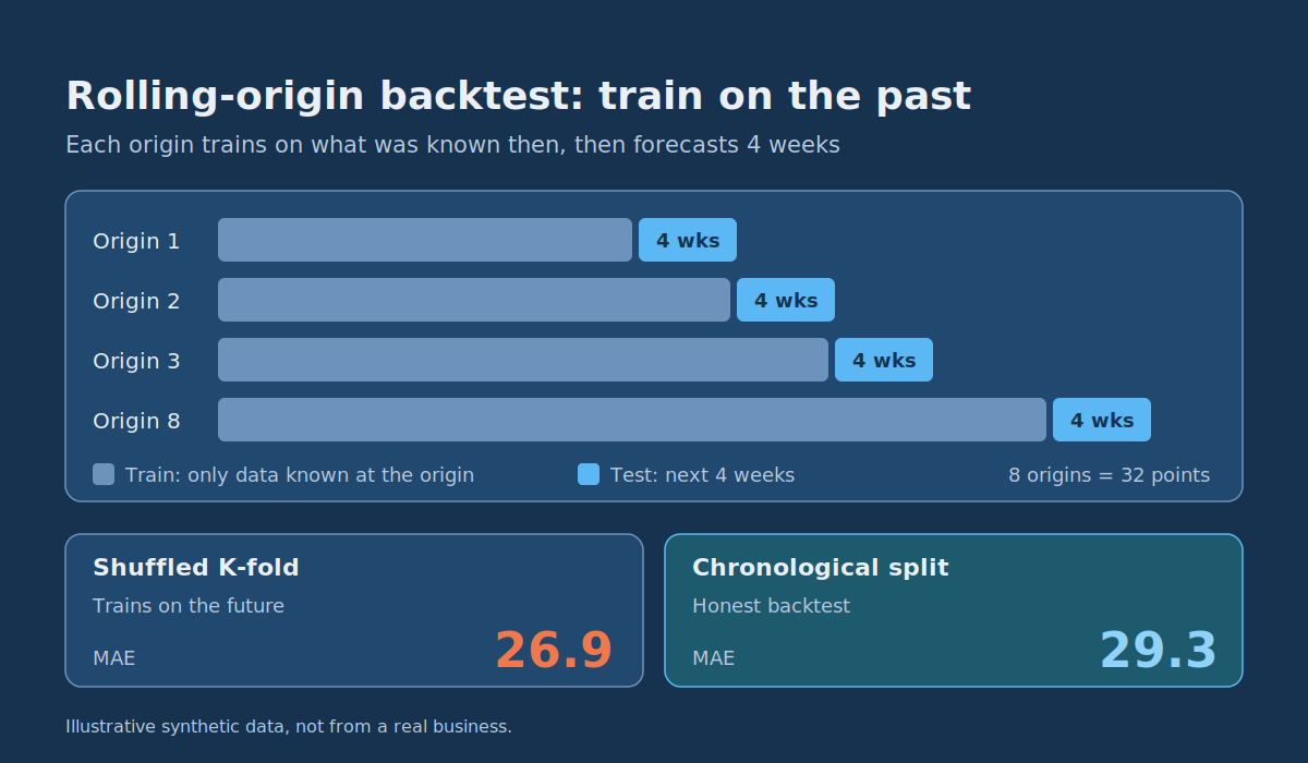
A backtest repeats the forecasting exercise at several past origins (the moment a forecast would have been issued), each time training only on what was known then and scoring the next few periods. This is often called time series cross-validation or rolling-origin evaluation, and the textbook Forecasting: Principles and Practice covers the idea in detail. It matters for three reasons: one test window can flatter or punish a model by luck, error typically changes with the forecast horizon, and the spread across origins tells you how much to trust the average.
The setup (illustrative example)
The data below is synthetic, not from a real business. It stands in for weekly unit demand for one product over four years, built from a slow upward trend (1.2 units per week), a yearly seasonal wave, a November promotion bump and random noise. The forecast spec is the one from earlier: 4 weeks ahead, issued weekly. The code compares three baselines with a gradient-boosted tree model that uses lag features, and also compares shuffled cross-validation with chronological folds. Swap the data-generation block for your own weekly series with a datetime index to adapt it.
import numpy as np
import pandas as pd
from sklearn.ensemble import HistGradientBoostingRegressor
from sklearn.model_selection import TimeSeriesSplit, KFold

# ---------- 1. Illustrative weekly demand: trend + yearly seasonality + noise ----------
rng = np.random.default_rng(42)
weeks = pd.date_range("2022-01-03", periods=208, freq="W-MON")   # 4 years
t = np.arange(len(weeks))
demand = (500 + 1.2 * t                                   # slow upward trend
          + 80 * np.sin(2 * np.pi * t / 52)               # yearly seasonality
          + 40 * (weeks.month == 11)                      # November promo bump
          + rng.normal(0, 25, len(weeks)))                # noise
y = pd.Series(demand.round(), index=weeks, name="units")

H, M = 4, 52                 # forecast horizon (weeks), season length (weeks)

# ---------- 2. Features that only use information available H weeks earlier ----------
X = pd.DataFrame(index=y.index)
for lag in (H, H + 1, H + 2, H + 4, M):                   # every lag >= H: no peeking
    X[f"lag_{lag}"] = y.shift(lag)
X["roll4_mean"] = y.shift(H).rolling(4).mean()            # shifted BEFORE rolling window
X["week_of_year"] = y.index.isocalendar().week.astype(int).values
valid = X.dropna().index                                  # drop rows lacking a 52-week lag
X, yv = X.loc[valid], y.loc[valid]

# ---------- 3. Metrics ----------
def mae(a, f):  return float(np.mean(np.abs(a - f)))
def wape(a, f): return float(np.sum(np.abs(a - f)) / np.sum(np.abs(a)))
def bias(a, f): return float(np.sum(f - a) / np.sum(a))
def mase(a, f, train, m):                                  # scaled by in-sample seasonal-naive error
    scale = np.mean(np.abs(train[m:] - train[:-m]))
    return float(np.mean(np.abs(a - f)) / scale)

# ---------- 4. Rolling-origin backtest: 8 origins, each forecasts the next H weeks ----------
tscv = TimeSeriesSplit(n_splits=8, test_size=H)
rows = []
for k, (tr, te) in enumerate(tscv.split(X)):
    train_y, actual = yv.iloc[tr].to_numpy(), yv.iloc[te].to_numpy()
    full_hist = y.loc[:yv.index[tr[-1]]].to_numpy()        # all actuals known at the origin
    naive   = np.repeat(full_hist[-1], H)                  # last value
    snaive  = full_hist[-M:][:H]                           # same weeks last year
    snaive2 = (full_hist[-M:][:H] + full_hist[-2*M:-M][:H]) / 2   # mean of last 2 years
    model = HistGradientBoostingRegressor(max_iter=200, learning_rate=0.05, random_state=0)
    model.fit(X.iloc[tr], train_y)
    ml = model.predict(X.iloc[te])
    for name, f in [("naive", naive), ("seasonal_naive", snaive),
                    ("seasonal_avg_2y", snaive2), ("gbm_lags", ml)]:
        rows.append(dict(fold=k, model=name, MAE=mae(actual, f), WAPE=wape(actual, f),
                         MASE=mase(actual, f, full_hist, M), bias=bias(actual, f)))
res = pd.DataFrame(rows)
print(res.groupby("model")[["MAE", "WAPE", "MASE", "bias"]].mean().round(3).sort_values("MASE"))

# ---------- 5. Leakage demo: shuffled K-fold vs chronological folds, same model ----------
def cv_mae(splitter):
    errs = []
    for tr, te in splitter.split(X):
        m = HistGradientBoostingRegressor(max_iter=200, learning_rate=0.05, random_state=0)
        m.fit(X.iloc[tr], yv.iloc[tr]); errs.append(mae(yv.iloc[te].to_numpy(), m.predict(X.iloc[te])))
    return np.mean(errs)
print("shuffled KFold MAE:   ", round(cv_mae(KFold(8, shuffle=True, random_state=0)), 1))
print("TimeSeriesSplit MAE:  ", round(cv_mae(TimeSeriesSplit(8, test_size=H)), 1))

# ---------- 6. Intermittent demand: why MAPE breaks ----------
spare = np.array([0, 0, 3, 0, 0, 0, 5, 0, 0, 2, 0, 0])
fc    = np.full_like(spare, spare.mean(), dtype=float)
with np.errstate(divide="ignore", invalid="ignore"):
    mape = np.mean(np.abs(spare - fc) / spare)
print("MAPE:", mape, "| MAE:", round(mae(spare, fc), 2), "| WAPE:", round(wape(spare, fc), 2))
This code was run once with Python 3.12, scikit-learn 1.8.0, pandas 3.0.2 and NumPy 2.4.4. Other versions, or a different random seed, may print slightly different numbers.
The output, and how to read it
                     MAE   WAPE   MASE   bias
model
gbm_lags          29.330  0.041  0.474 -0.011
naive             38.656  0.055  0.622 -0.001
seasonal_naive    69.688  0.099  1.128 -0.097
seasonal_avg_2y  100.172  0.143  1.621 -0.143
shuffled KFold MAE:    26.9
TimeSeriesSplit MAE:   29.3
MAPE: inf | MAE: 1.25 | WAPE: 1.5| Method | MAE (units) | WAPE | MASE | Bias |
|---|---|---|---|---|
| Gradient-boosted trees on lags | 29.3 | 4.1% | 0.47 | −1.1% |
| Naive (last value) | 38.7 | 5.5% | 0.62 | −0.1% |
| Seasonal naive | 69.7 | 9.9% | 1.13 | −9.7% |
| Average of last two years, same weeks | 100.2 | 14.3% | 1.62 | −14.3% |
Several things stand out. First, the two seasonal baselines lose badly, and their bias column shows why. Both are persistently low, by about 10% and 14%, because they carry old levels into a series that grows by roughly 62 units a year. A seasonal baseline is not automatically the safer baseline when there is a trend. Second, plain naive is hard to beat on a 4-week horizon: it is essentially unbiased and sits well below the seasonal methods. Third, the tree model beats it by about 24% on MAE and does so with almost no bias, which is the result you want before accepting extra complexity.
Fourth, shuffled K-fold reported 26.9 against 29.3 for the chronological backtest on the same model and features. On this smooth series the flattery is modest, around 8%, and the direction matters more than the size. Real series with level shifts or promotions often show larger gaps, but that is an expectation, not something these numbers prove. Finally, remember the sample is small: eight origins of four weeks each is only 32 forecast points. The gaps above are large enough to be meaningful, but if two methods land within a few percent of each other, you would need many more origins before declaring a winner.
Forecast accuracy metrics: MAE, WAPE, MASE and bias
No single metric is correct everywhere. MAE is easy to explain in units. WAPE (weighted absolute percentage error) divides total absolute error by total actual volume, so it gives a percentage that isn’t dominated by tiny periods. MASE (mean absolute scaled error), proposed by Hyndman and Koehler in 2006, divides your error by the average error of a naive benchmark on the training data, which lets you compare series with different scales. A MASE below 1 means your errors are smaller than that benchmark’s typical in-sample error, so it is a useful ruler but not the same thing as beating the benchmark out-of-sample. In the example above, seasonal naive scores 1.13 on the test windows because of the trend, even though the scale itself came from training data. Bias, the signed total error as a share of actuals, tells you whether you are systematically over- or under-forecasting, which the other metrics hide.
| Situation | Prefer | Why | Watch out for |
|---|---|---|---|
| One series, stakeholders want plain language | MAE and WAPE | MAE is in real units; WAPE is a single percentage of total volume | Both can hide a steady under- or over-forecast, so add bias |
| Many series on different scales (hundreds of SKUs) | MASE per series, WAPE for the portfolio | MASE is scale-free; WAPE weights by volume so big sellers count more | MASE is undefined if the training series is constant |
| Actuals include zeros or near-zeros | MAE, WAPE, MASE | Percentage errors divide by the actual, which fails at zero | Avoid MAPE; the code above prints inf for it |
| Intermittent (lumpy) demand | Metric chosen from the decision, plus bias | MAE rewards forecasting zero; squared-error metrics reward forecasting the mean, so they pull in different directions | A single point forecast may be the wrong object; consider forecasting a service-level quantile instead |
| Large misses are disproportionately costly | RMSE alongside MAE | Squaring punishes big errors more | One outlier week can dominate the score |
| Over- and under-forecasting cost different amounts | Bias plus a cost-weighted error | Symmetric metrics treat a stockout and an overstock the same | You need an honest estimate of the two costs |
The last output line of the code shows the intermittent case concretely. With a spare-parts series that is mostly zeros, MAPE is infinite because it divides by zero actuals, while MAE and WAPE remain well defined. There is a subtler trap too: for such a series, forecasting zero everywhere produces a lower MAE (about 0.83) than forecasting the average (1.25), even though a forecast of zero would leave you with no stock. When demand is lumpy, choose the metric from the decision you are supporting rather than from habit, and consider reporting at a coarser time bucket, since monthly totals are far less sparse than daily counts.
Choose between a baseline, classical statistics and machine learning
Use the backtest to make this choice rather than preference. As a working rule:
- Stay with a baseline when no candidate beats it consistently across origins and horizons, or when the improvement is smaller than the noise between folds. A baseline is cheap to run, easy to explain and hard to break.
- Use classical statistical models (exponential smoothing, ARIMA variants) when you have a modest number of series, a clear trend and seasonal pattern and little or no external driver data. They need little feature work and handle trend and seasonality directly.
- Use machine learning when you have many related series, useful drivers such as promotions, price or calendar effects, and enough history to learn from. The cost is more feature engineering, more leakage risk and more to monitor. If a backtest shows a model is worth building, you can create a machine learning model fast, as long as it is benchmarked against the baselines first, as the worked example above was.
- Choose nothing yet if even the best method has an unacceptable error for the decision it supports. A forecast that is no better than a baseline, or whose error exceeds the tolerance of the decision, shouldn’t go into a planning process.
From backtest to deployment
A backtest tells you how a method would have behaved in the past. Deployment is where it can still go wrong. Rebuild the exact feature pipeline used in the backtest, with the same lags and the same issue time, and make sure each feature is available when the forecast runs. Store every forecast with the date it was issued, so you can later compare it with actuals without hindsight. Track live error against the backtest range, including bias, and set a trigger for retraining or review when it drifts outside it. Retrain on a schedule that matches how quickly the series changes, and keep the best naive or seasonal naive forecast running alongside the model as a fallback and a permanent yardstick. If the model stops beating the baseline in production, you want to see that quickly.
Getting the forecast into the tools people actually use matters as much as the model. If your planners still copy numbers between spreadsheets, custom software development for business workflows can connect the forecast, its issue date and its error tracking directly to the ordering or scheduling process it supports.
Next step: test your own forecast
Take one series you forecast today, write down its grain, horizon and issue time, and run the naive and seasonal naive baselines through a rolling-origin backtest using the code above. The result is a defensible starting point for deciding whether anything more elaborate is justified. If you would like a second opinion on whether your operational data can support a useful forecast, DataColab can discuss a forecasting feasibility assessment on a sample of your real data before any build begins.